How LLMs Work, From Scratch

When ChatGPT launched in late 2022, it opened a whole new set of possibilities for what computers can do. Fast forward to today, AI has already started contributing to the world in many ways, from writing code to speeding up scientific progress. Over the past few years AI models have kept getting better, and so has everything you can do with them.

And yet, most of us still don't know how this technology actually works.

A Large language model, is simply just a mathematical function: given some input text, it predicts the probability of what word comes next. I wanted to understand how LLMs work from scratch, not to become an expert, but to understand the basics of this technology.

In this post, I've broken down every step of how LLMs work from scratch, stripping away the complexity. By the end, you should have a simple mental model for how LLMs work fundamentally.

1. Tokenization

LLMs are mathematical functions; they don't understand words. We need a way to convert words to integers using a process called Tokenization.

1. Tokenization breaks down text into smaller units called tokens.
2. Each token is then mapped to a numerical value (Token-ID) that the model can process.

For instance: take a small dataset of 500 US names. You can map all characters in the alphabet to an integer:

Token ID	Character
0	a
1	b
2	c
…	…
25	z
26	special token

Now any name is a list of integers. SID → [19, 8, 3], JOHN → [10, 15, 8, 14].

This was a simple example, but in today's LLMs, instead of mapping each character to a token ID, models use subword tokenization techniques. Why?

1. Human language is fairly complex. Splitting tokens into subwords lets the model handle words it never saw in training by assembling them from pieces.
2. Models don't use character-to-token mapping because it makes sequences long and slow to compute.

Currently, Frontier Labs uses subword tokenization techniques like Byte Pair Encoding (BPE). BPE starts with individual characters and iteratively merges the most frequent pairs of symbols to form new tokens.

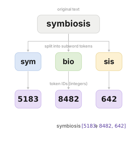
Alongside the regular tokens in the dataset, models add tokens for structure.

• BOS (beginning of sequence) sits at the start, so the first real token has something before it to look at.
• EOS (end of sequence) sits at the end. During inference, producing an EOS is the signal to stop. Without it, the model runs forever.

Some models use one token for both jobs. For example, a name will be represented as [BOS, S, I, D, EOS]

The model now has a predefined vocabulary of words with an integer value attached to each entry.

2. Embedding: giving tokens meaning

Token IDs are arbitrary integers; they don't have any meaning.

a = 0, b = 1…

The numbers mean nothing by themselves. We need a way to give meaning to these tokens.

Embeddings fix this.

Picture a library where each book (words) has a barcode (token-ID) stuck on it. The barcode says nothing about the book. What you actually want is a description: topic: food, difficulty: easy, language: english. An embedding is that description, written as a vector of numbers.

Embedding is a learned vector of numbers that stores information about the token, for the model to do math on it.

Word-Token-Embedding

Every model keeps an embedding matrix. Every token ID has a vector associated with it. For instance, take a small vocabulary with a 3-dimensional embedding vector; an embedding matrix for it looks like this (showing just a few tokens):

Token ID	Token	Embedding vector
0	"cat"	[0.9, 0.1, 0.8]
1	"kitten"	[0.85, 0.15, 0.75]
2	"car"	[0.1, 0.9, 0.2]

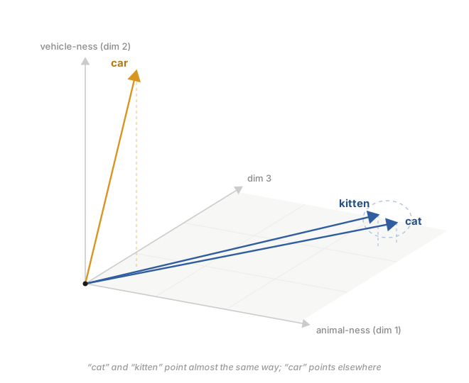
For instance, in this example you can see:

“cat” [0.9, 0.1, 0.8] and “kitten” [0.85, 0.15, 0.75] are very close in the 3-D space. While “car” [0.1, 0.9, 0.2] is far away, even though its ID (2) is right next to cat's (0).

The embedding vector encodes meaning about the token that is learned in the training process. Maybe the first dimension captures “animal-ness,” the second “vehicle-ness.” Nobody set them by hand. The model learned them.

Because the vectors hold meaning, something surprising happens. After training, you can do meaningful arithmetic on tokens:

vec("king") - vec("man") + vec("woman") ≈ vec("queen")

Nobody coded that. It fell out of training.

This embedding matrix is called WTE (word token embedding) matrix. The dimension of the WTE matrix is (no. of token IDs, dimension of embedding), which is (50257, 768) for GPT-2.

Word-Position-Embedding

Let's take two sentences:

“The dog bit the man”
“The man bit the dog”

Both snippets have the same tokens, but the order of tokens changes the meaning completely.

The embedding vector for “man” in both cases is the same. We need a way to add the positional meaning to each vector.

The fix is a second matrix, WPE (word position embedding).

For instance, take a model with a context window (the maximum tokens an AI model can process in a single request) of 5 tokens, with a 3-dimensional position embedding vector; the WPE looks like this:

Position	Position vector
0	[0.00, 0.10, 0.00]
1	[0.30, 0.20, 0.40]
2	[0.10, 0.40, 0.60]
3	[0.85, 0.12, 0.50]
4	[0.15, 0.45, 0.75]

The dimension of the embedding vector is (context window × dimension of embedding vector). GPT-2's WPE is (1024, 768).

The input to the next transformer block is just the two added together:

Xi = WTE[token]  (what it is)
   + WPE[i]      (where it sits)

For “dog” sitting in position 1, the final embedding vector that gets passed to the next stage is:

X(dog) = [0.8, 0.2, 0.7]   (its WTE embedding)
       + [0.0, 0.1, 0.0]   (the position-1 vector from WPE)

Now “dog” in position 2 and “dog” in position 5 look different, and word order finally means something.

3. Attention

Now we have an input X per token that encodes its meaning and position.

Consider this example:

“She walked to the river bank to fish.”
“She called her investment bank about the loan.”

The token ‘bank’ has the exact same embedding vector, but it means completely different things in both examples. A fixed vector can't be both a riverbank and a financial one.

The model needs a way to update its vector to encode information from its surroundings. If the token ‘bank’ is near “river” and “fish,” it should lean geographic.

It's the job of the Attention Block in the Transformer where the tokens communicate with each other to update their values based on context. Figure out which earlier tokens are relevant and what to add to X(bank) to produce a refined X′(bank) that encodes the meaning of the words that came before it.

Attention is the trickiest concept to wrap your head around in this blog. Let's take the phrase “her investment bank”. Here's how Attention works in 3 parts:

1. Query (Q): “bank” asks, who can help me predict the next token.
2. Key (K): every other token before ‘bank’ in the model's context presents its offer.
3. Value (V): the actual information the other tokens in context hand over once picked.

Now the mechanics.

Attention introduces three learned matrices, W_q, W_k, W_v, and each token multiplies its X by them to produce three vectors.

A quick note before we dive in: an attention head is just one independent copy of this whole Q, K, V machinery. A model runs many heads in parallel, each learning to look for a different kind of relationship.

Note

A dot product is a single number that measures how much two lists of numbers agree. You multiply them position by position and add it up, so [1, 2] and [3, 1] give 3 + 2 = 5. The idea is that a bigger number means the two lists are more alike, which is how a token measures how relevant another token is to it.

Softmax is a function that converts raw scores into probabilities. It takes any list of numbers like [1, -2, 3] and turns it into a distribution like [0.12, 0.01, 0.88], where every value sits between 0 and 1 and they all sum to 1. Crucially, it preserves the relative order: the highest score stays the highest and the lowest stays the lowest, so nothing gets reshuffled, it just gets rescaled into "how much attention goes to each token."

Step 1: Project into Q, K, V.

Every token's embedding vector X(bank) gets multiplied by three learned weight matrices, W_q, W_k, W_v, each of size (embedding dimension × head dimension), e.g. in GPT-2, each head's matrices are (768 × 64):

Query = X · Wq
Key   = X · Wk
Value = X · Wv

We calculate the Q, K, V vectors for every token in the context.

Step 2: Compute attention scores: take the dot product of each Query with every Key to get a score matrix:

Q \ K	her	investment	bank
her	2	0	1
investment	0	2	1
bank	1	3	1

The highlighted row is the one we follow, the Query "bank" against every Key.

For “bank”, the raw scores are [1, 3, 1]: it aligns strongly with “investment”, weakly with “her” and with itself.

Step 3: Scale: these scores can get large, so we divide by √(d_k), the square root of the head dimension — the length of each Q/K/V vector. In this toy example each head is 3-dimensional, so d_k = 3 and √(d_k) = √3 = 1.73. This keeps gradients stable.

[1, 3, 1]  → ÷ √(dk) = ÷√3 →  [0.57, 1.73, 0.57]

Step 4: Convert to probabilities: run the scaled scores through softmax so they sum to 1.

[0.57, 1.73, 0.57]  → softmax →  [0.2, 0.6, 0.2]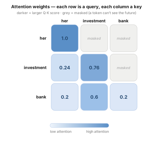

Step 5: Weighted sum of Values: multiply each token's Value vector by its attention weight and sum:

0.2 × V("her") + 0.6 × V("investment") + 0.2 × V("bank") = new context-aware vector for "bank"

The whole thing in one line:

Attention(Q, K, V) = softmax(Q · Kᵀ / √dk) · V

Before attention, “bank” was just “bank”, the same vector in a riverbank sentence or a finance one. After, it's “bank, mostly shaped by ‘investment’,” already leaning financial before the model predicts a single word. The vector wasn't replaced. It got nudged toward the meaning its neighbors imply.

Causal Masking (No peeking)

There's one flaw in Attention. A token may only attend to itself and what came before it. Otherwise it's cheating. We enforce this by setting future scores to negative infinity before softmax (e^-∞ = 0), which makes their probability zero:

Q \ K	her	investment	bank
her	0	−∞	−∞
investment	0	0	−∞
bank	1	3	1

“her” sees only itself. “investment” sees “her” and itself. “bank” sees everything before it. Every token predicts using only the past, exactly as it will when generating for real.

Multi-head attention

One head learns one kind of relationship. Language has many at once, so we run several in parallel, each with its own W_q, W_k, W_v, each hunting a different pattern.

The trick is to split the vector into equal chunks, one per head, instead of handing each head the full width. In GPT-2, for example, a 768-dimension embedding vector X splits across 12 heads, taking 64 dimensions each.

Take a 4-dimension X(bank) vector with 2 heads:

"bank": [0.9, 0.1, 0.8, 0.2]
Head 1: [0.9, 0.1]      Head 2: [0.8, 0.2]

Each head runs the five steps above on its own slice. One might lean on grammar (“bank” is a singular subject), the other on meaning (“bank” is related to finance). Say they come back with:

Head 1 → [0.67, 0.67]
Head 2 → [0.16, 0.58]

Glue them back together, up to full width again (4 here):

[0.67, 0.67, 0.16, 0.58]

One last matrix, W_o, mixes the glued heads together to get the final result.

[0.67, 0.67, 0.16, 0.58] × Wo = [0.8, 1.1, 0.4, 0.9]   ← final attention output for "bank"

4. Feed Forward Network (MLP)

The next block is the MLP (or feed-forward network), this is the part where LLMs store facts. In the previous step, the token ‘bank’ gathered context from the surrounding tokens, but it still hasn't reasoned through it.

Knowing “river is near” and “bank is near” isn't the same as concluding “this is geography.” To reason over the fact that river + bank = riverbank, models need a thinking layer, and that's where MLPs help.

MLP stands for multilayer perceptron. In this layer, each token's embedding vector goes through a series of operations where it expands to a larger dimension first and then compresses back to its initial dimension.

Unlike the previous step where each token ‘attends’ to one another, in this step each token thinks on its own. No token talks to another here; they all run the same operation in parallel.

Here's the working:

1. Expand (W₁). Blow the vector up into a bigger space (GPT-2 goes 768 → 3072) by multiplying it with the W₁ matrix.
2. Apply a nonlinearity like GeLU, ReLU, etc.
   The simplest nonlinear function example is ReLU, which just zeroes out negatives and passes positives through: [0.8, 1.4, -0.2, 2.1] (ReLU) → [0.8, 1.4, 0, 2.1]
3. Compress (W₂). Multiply by the W₂ matrix to shrink back to the original size.

Mathematically:

MLP(x) = W2 · GELU(W1x + b1) + b2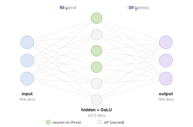

A nice way to read it: each row of W₁ asks one question (“is this river + bank?”). The answer after the nonlinearity is a neuron: positive for yes, zero for no. Each column of W₂ is the response to add back when that neuron fires. When “riverbank” lights up, W₂ stamps “geography, water, landscape” onto the token.

This is also where facts live. Most of a model's parameters sit in these layers, not in attention, and they aren't generic bookkeeping. Researchers have found single neurons that fire on the Eiffel Tower, or on past-tense verbs, or on a specific programming language. When a model “knows” Paris is the capital of France, that fact is spread across FFN weights in particular layers.

5. LayerNorm and Residuals

Two pieces of plumbing keep a deep stack trainable.

LayerNorm. After a few blocks, a token's numbers drift. Some hit 500, others 0.001. Softmax hates that ([500, 501, 499] collapses to nearly [0, 1, 0]), and training goes unstable. LayerNorm rescales each token's vector to mean 0 and spread 1, keeping the pattern but taming the scale. [10, 2, 6, 14] becomes [0.45, -1.34, -0.45, 1.34] Notice how the relative pattern is preserved but the scale is tamed.

Residuals. Each block adds its output back onto its input instead of replacing it:

new = old + block(old)

Without this, a later block can wipe out what an earlier one figured out, and “bank” could forget it was ever “bank.” With it, the original rides along and each block only has to add a small nudge. A block with nothing useful to contribute can output roughly 0 and get skipped for free.

For instance, “cat”'s vector is [0.8, 0.3] and attention produces the update [0.0, 1.1]:

• Without residual: new vector = [0.0, 1.1], the 0.8 is gone forever, unrecoverable by later blocks.
• With residual: new vector = [0.8, 0.3] + [0.0, 1.1] = [0.8, 1.4], the original survives, new context layered on top.

Residuals also save training. A deep stack has to send a correction signal backward from the last block to the first, and without a shortcut that signal fades to nothing on the way. This is the vanishing gradient problem. The residual is a clean path straight through, so early layers still learn. More on that in part 2.

LayerNorm and Residuals are added after each block to keep the model trainable.

6. The Full Forward Pass

We've built every piece on its own. Now let's wire them together and watch a single token make the whole trip.

One forward pass is just text going in one end and a prediction coming out the other. Tokenize the text, look up each token's meaning and position, then push the stack through the transformer blocks: attention lets the tokens read each other, the MLP reasons over what they gathered, and LayerNorm and residuals keep the whole thing stable. That block repeats over and over (12 times in GPT-2), each pass layering a little more context onto every token.

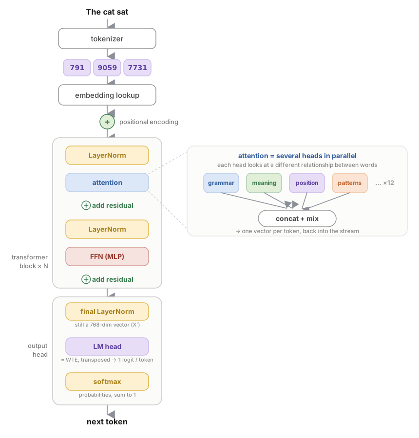
We've followed a token all the way from tokenization through the transformer blocks. Out the far end comes a refined vector X′, loaded with all the context it gathered along the way. But X′ is still just a list of numbers. We need to turn it back into words and predict the next token, the job we started with. Three steps do it:

1. A final LayerNorm. One last rescale to tidy up the vector. We're still left with a 768-dimensional embedding vector (in GPT-2), the same shape we started with back in the embedding step.
2. The language-model head (LM head). To get from a vector back to words, we do the reverse of embedding: embedding turned a token ID into a vector, now we turn a vector into a score for every token in the vocabulary. We don't even need a brand-new matrix, the head is usually the embedding matrix (WTE) transposed, a (768 × vocab) matrix reused in reverse. Multiplying X′ by it gives one raw score per token. Those scores are the logits.
3. Softmax. Turn the logits into probabilities that sum to 1. That's the probability table from the top of the post.

Back to our sentence, “She called her investment ___”. The LM head turns X′ into one logit per token in the vocabulary, and softmax turns those into probabilities:

Token	Logit	Probability
bank	3.4	0.61
firm	2.4	0.23
advisor	1.6	0.10
account	0.5	0.03
loan	-0.2	0.02
broker	-0.4	0.01

The model is most confident the next word is bank. One logit per token, squashed into one probability per token, and the highest one is the model's best guess. (The names model works the same way, just with vocab = 27, one score for each letter a to z plus the end token.)

Here's the whole forward pass in code:

def gpt(token_ids, positions):
    x = wte[token_ids] + wpe[positions]   # embed: what + where

    for block in blocks:                  # 12 blocks in GPT-2
        x = x + attn(layer_norm(x))       # gather context (+ residual)
        x = x + mlp(layer_norm(x))        # reason over it (+ residual)

    x = layer_norm_final(x)
    return lm_head(x)                     # logits over the vocabulary

That's the forward pass. Embed the tokens, alternate attention and MLP a dozen times, project back to the vocabulary. Every section above is one line here.

Inference

The model scores every position at once, but when generating we only care about the last one: the prediction for the next token.

Generation is a loop. Predict a token, stick it on the end, run again.

"She called her investment" → "bank"
"She called her investment bank" → "about"
...

How you pick from the distribution is a choice:

• Greedy: always take the top token. Deterministic, often dull.
• Temperature: divide the logits by T before softmax. Below 1 sharpens the odds (safer), above 1 flattens them (wilder).
• Top-k / top-p: sample only from the top k tokens, or from the smallest set of tokens covering probability p.

You stop when the model emits EOS, or when you hit a length cap. The names model samples letters (s, a, m) until it emits the end token, and you've got a fresh name.

What Next?

It took decades of breakthroughs in computer science to finally build AI, and there's still so much left to do. What we covered here is just the foundation, there's a lot more to how LLMs work, at scale and in optimization, that I didn't get into. But hopefully these basics open up the vast ocean of things you can now go learn from.

The best next step is to see all of this in code. Go read microGPT, the whole thing running in a couple hundred lines of Python.

If you found this helpful, reach out on X. I'd love your feedback, and I love making new friends.

This post was inspired by Karpathy's microGPT and blog, Lee Robinson's Understanding AI, and 0xkato's How LLMs Actually Work.